Simple Inverter Circuit

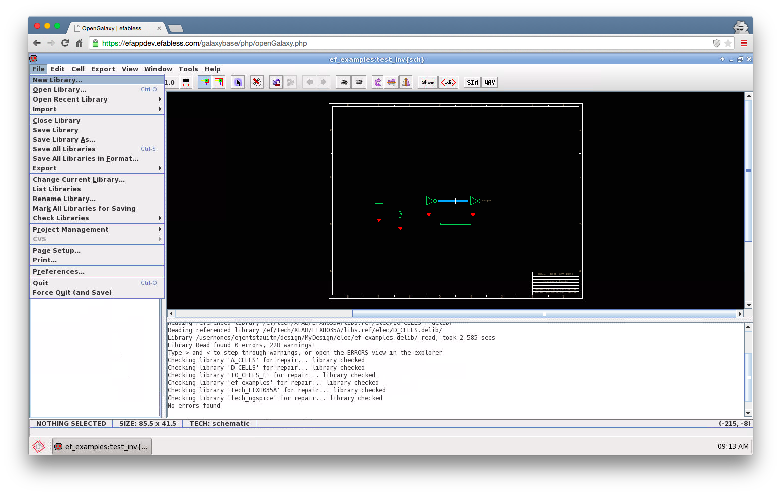
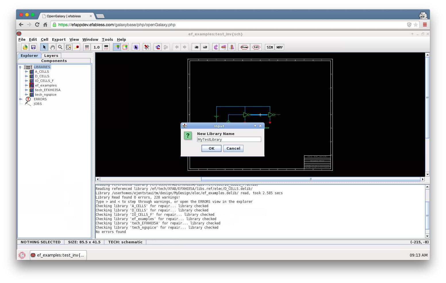
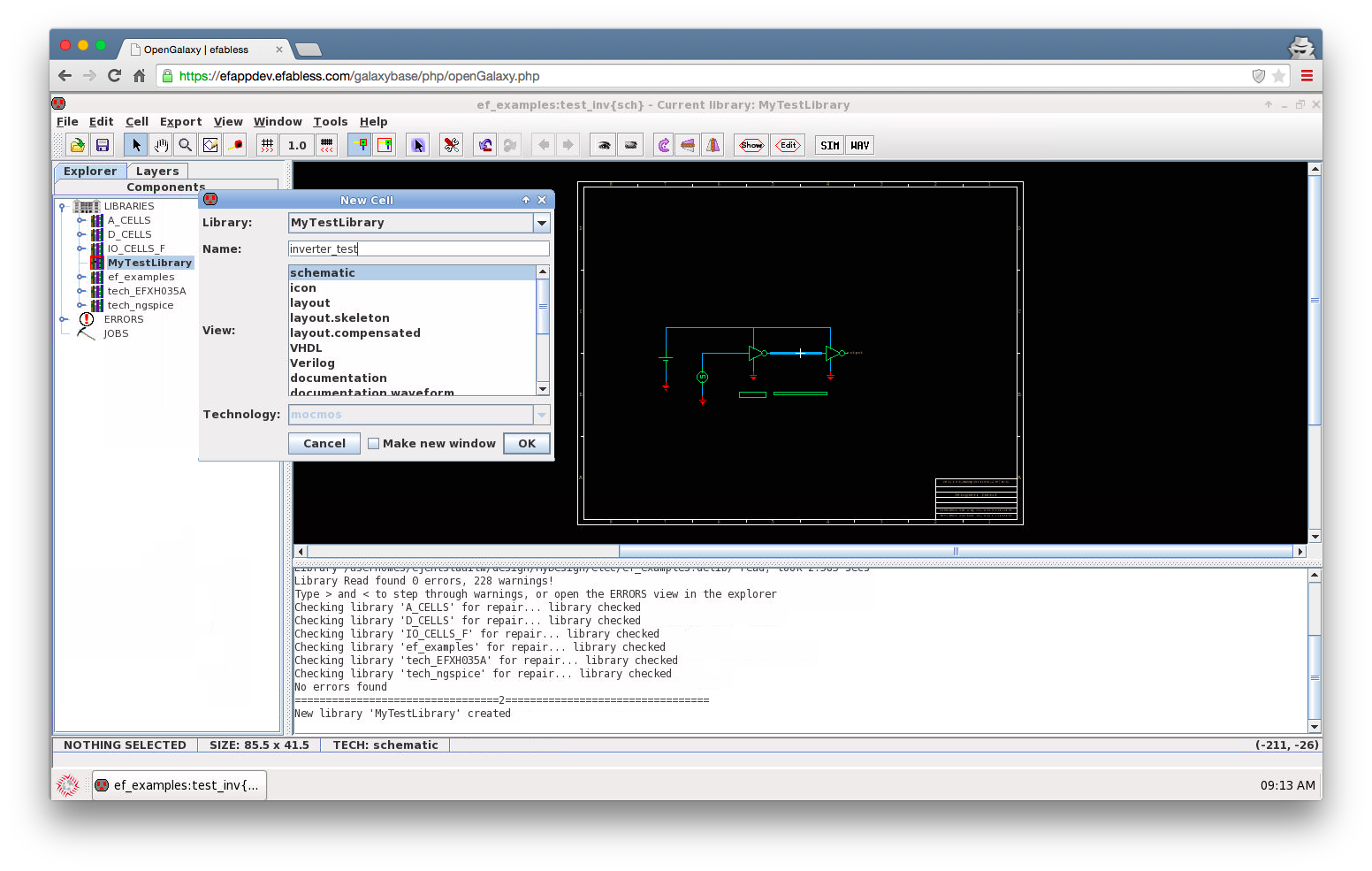
Let’s start Electric and create a new library, call it ‘MyTestLibrary’

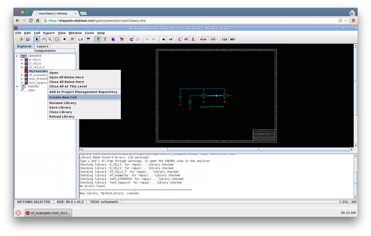
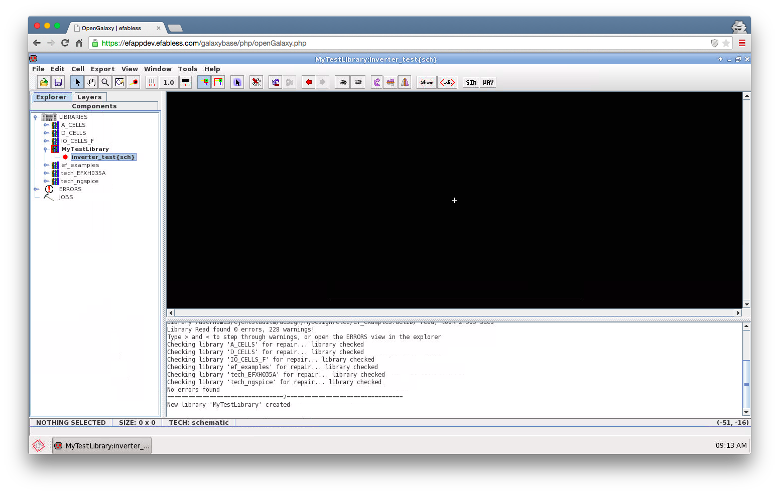
Then we can create a new cell inside MyTestLibrary. Let’s create an inverter, we have to create the schematic view of the cell (right click the libraryName in Explorer to pop-up the context menu)

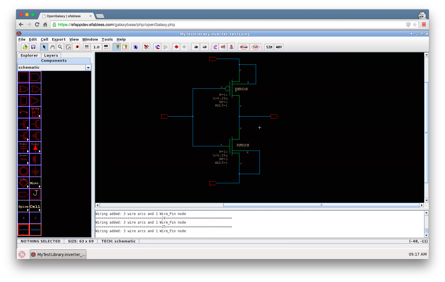
We can instantiate devices into the schematic by dragging from the libraries in the Explorer bar (on the left). We can instantiate primitive devices, IP blocks, any cell that has an ‘icon’ view (we’ll come to that later). For now we start by placing transistors, in this case we drag an ‘nmos’ and a ‘pmos’ into the sheet from libraryName tech_EFXH035A.

If tech_EFXH035A is not open in Explorer, find and open it using File/Open Library, it should be shown as-if in your current elec/ dir but with a “[REF]” suffix. For more on this see: Create a schematic

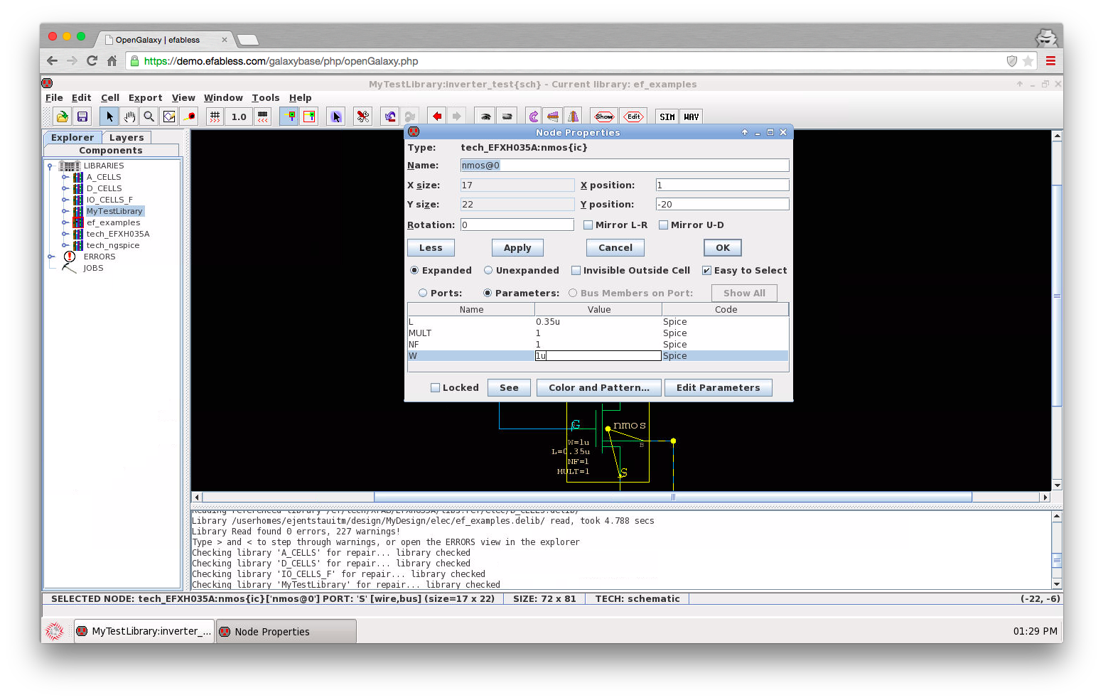
To edit any device parameter, double click on the device (the nmos in that case), a properties window will appear, make sure the ‘Parameters’ radiobox is selected.

Wire the devices (start at one terminal with a left click, then right click the other terminal), in the side-bar at left select the ‘Components’ tab, then drag ports into the schematic to add pins to the inverter. These pins are used to construct a symbol of the inverter and allow using it hierarchically in other schematics.

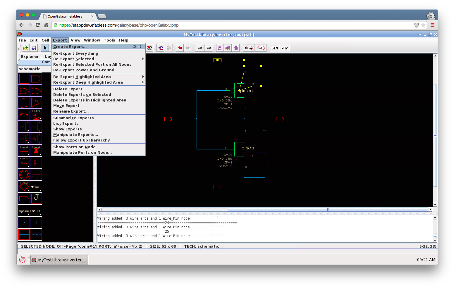
Now every red pin doesn’t have an ‘Export’ associated with it. In Electric it’s not enough to just add a pin to the net, you have to define an export that represents the electrical connectivity to the pin which can be propagated to higher levels in schematics. To add an export to the pins simply select the specific pin, then select Export/Create Export …

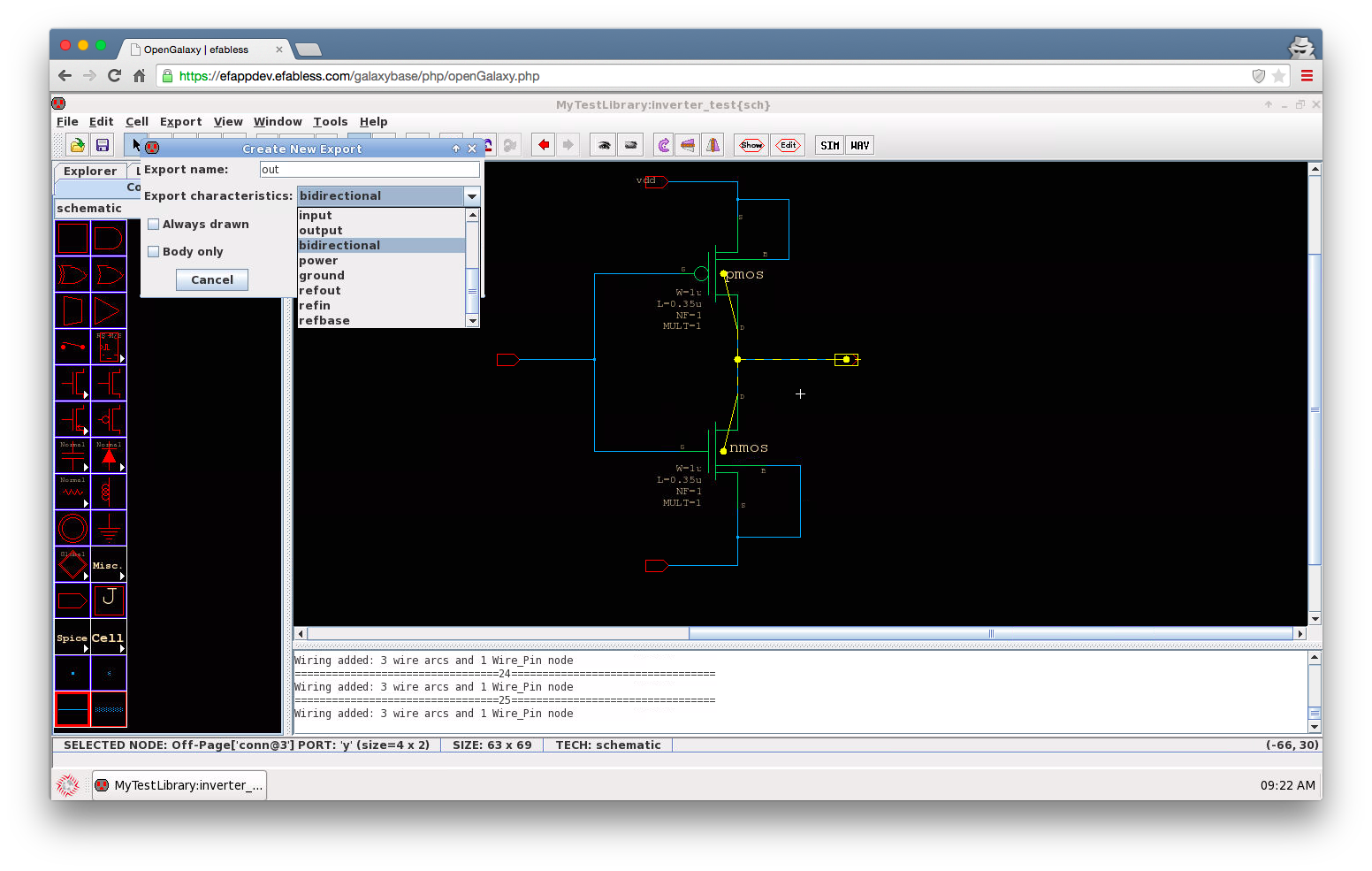
When the dialog box pops up type in the name of the export, choose the proper export characteristic (in, out, bidirectional) Note: Directional characteristic only matters when creating verilog netlists of the schematics, but it also nicely changes the schematic pin shape accordingly.

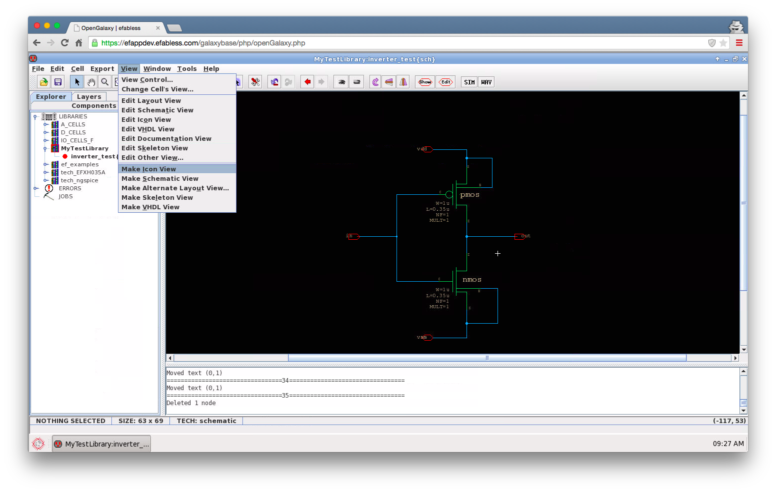
After completing the inverter schematic and adding proper exports to pins, it’s time to create an ‘icon’ view (which is a symbol that allows using the inverter in other schematics). Go to View/Make Icon View

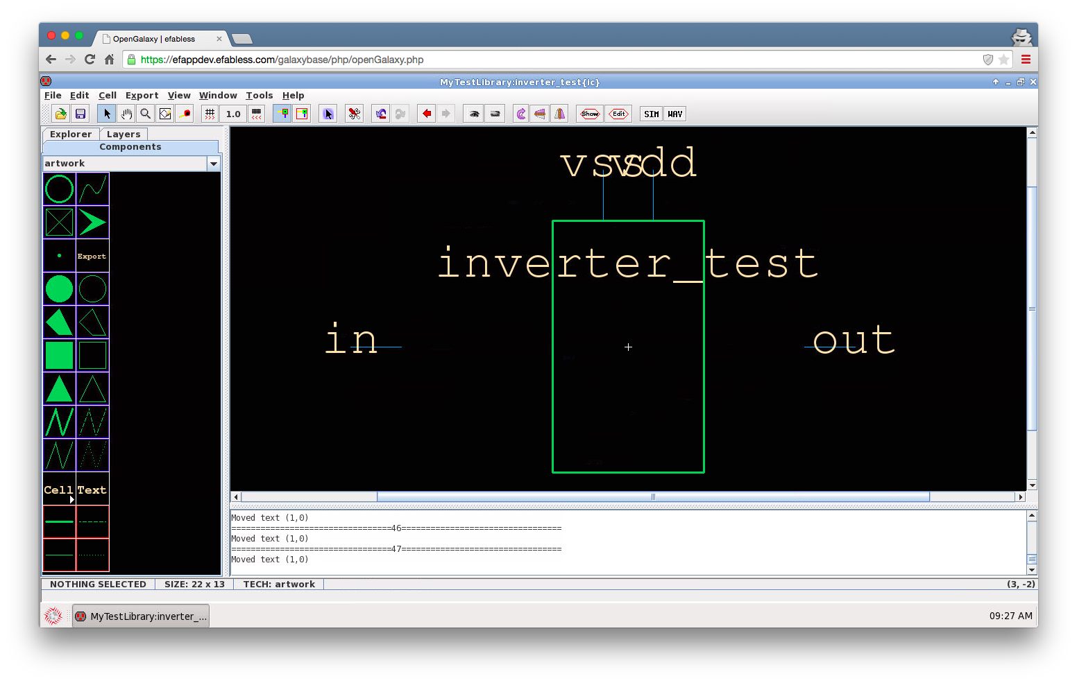
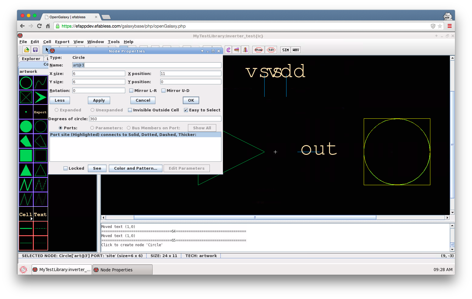
This will automatically create a boxed symbol of the inverter. To edit the icon simply double click on the icon view in the side-bar Explorer tab, then you can edit the icon, move around the pins, create other shapes (form the ‘Components’ tab on the left)

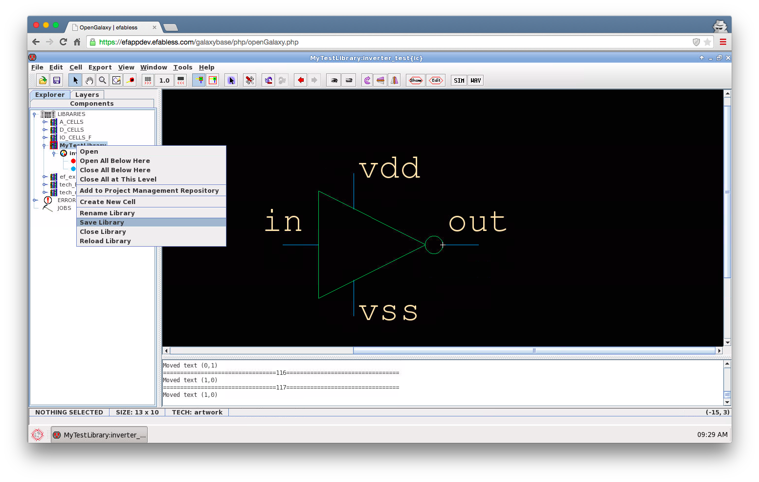
After completing the icon edits you probably want to save your changes, to save changes in Electric you have to save the whole library, in the side-bar Explorer tar at left, right-click the library to save (highlighted in bold, means that there are unsaved changes in some of the cells) then select ‘Save Library’. For more see: Save Electric working library

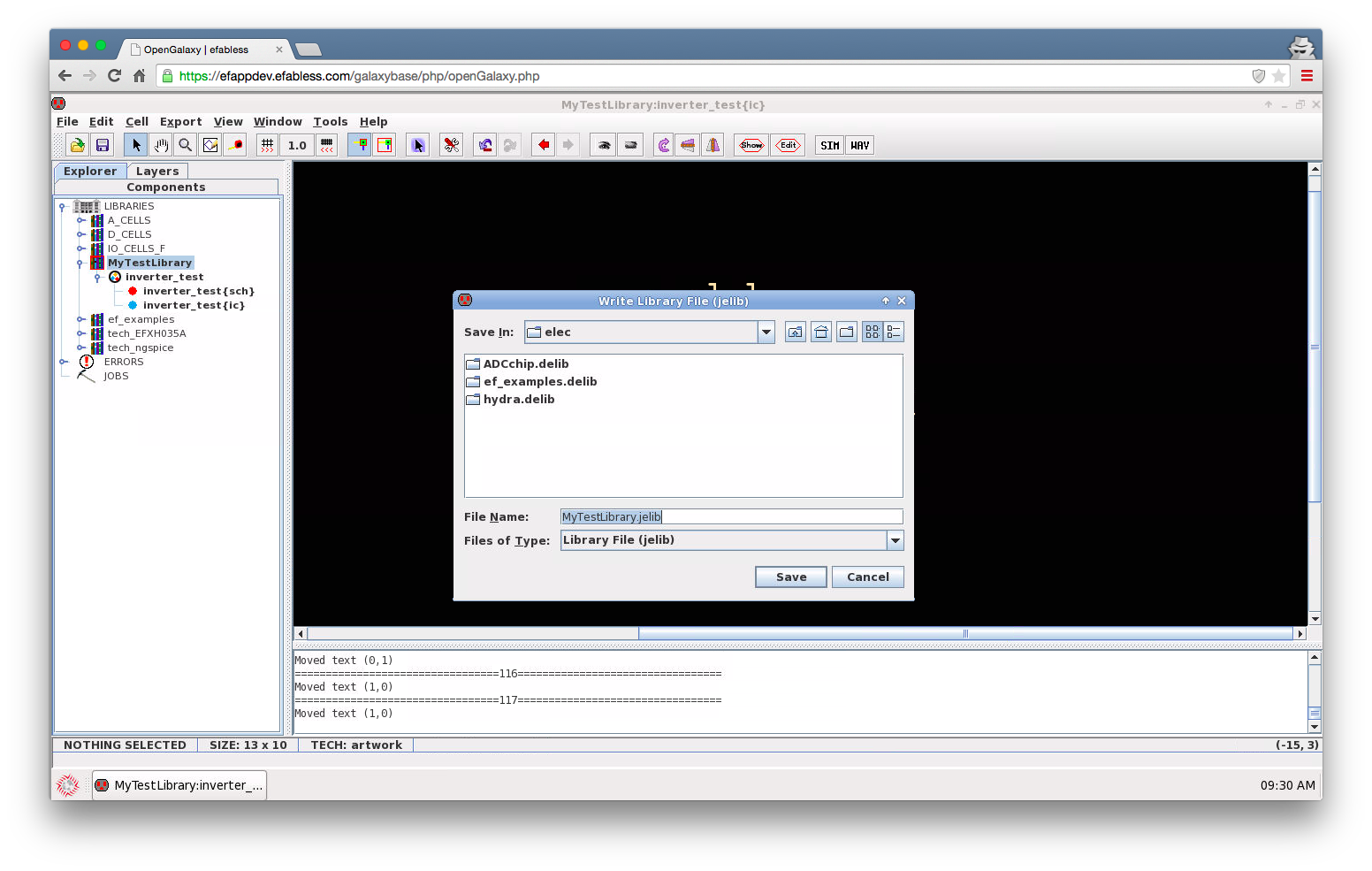
If this is the first time you’re saving the library you will be prompted to select a directory name and path in which the library will be saved. The name should be the same as the library name with a .delib extension, in this example it is ‘MyTestLibrary.delib’, the location should be inside the ‘elec’ directory which is inside the project directory.

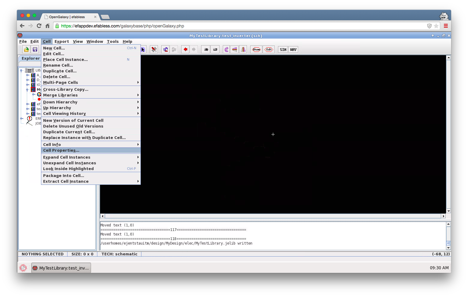
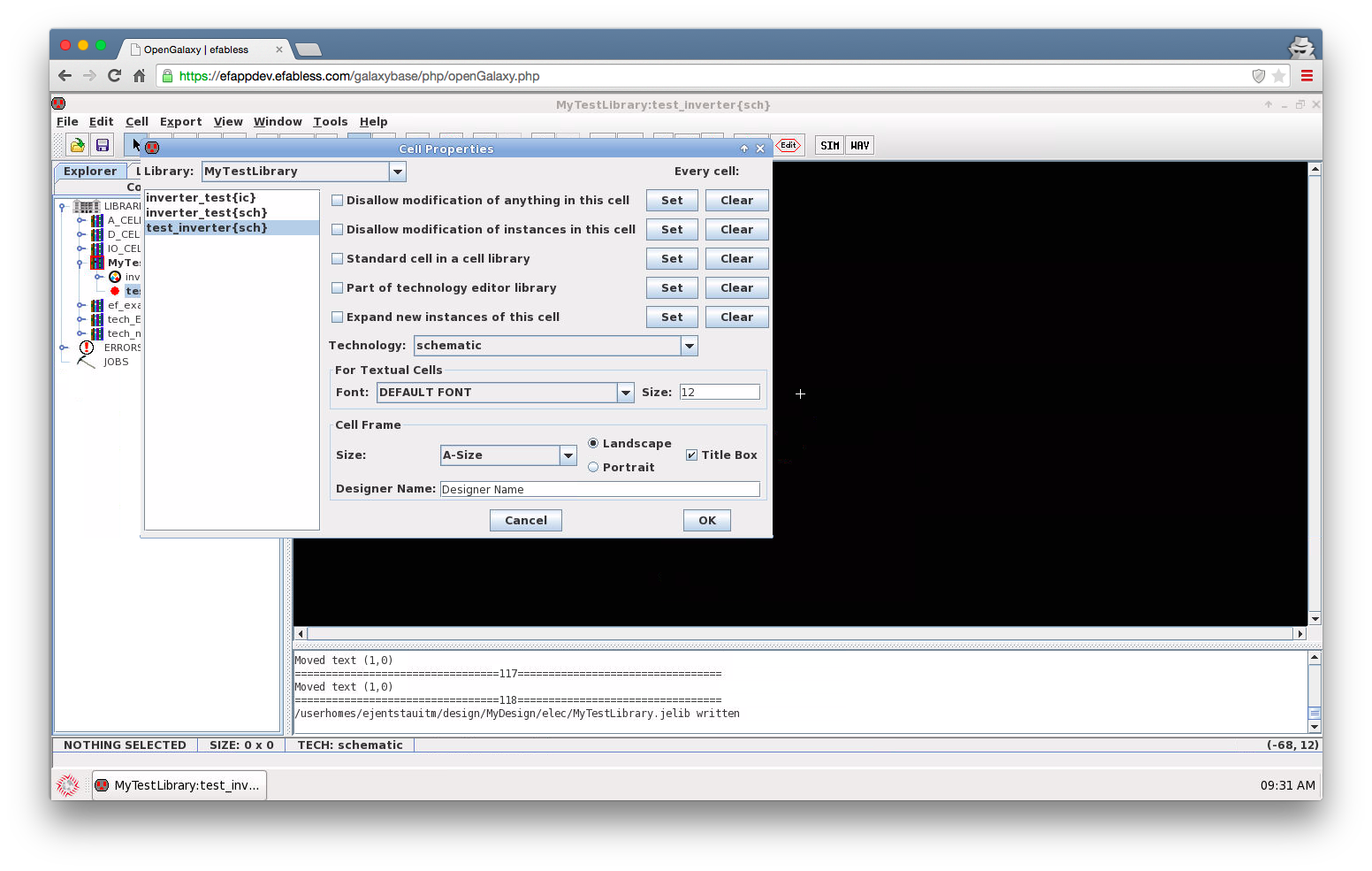
Now create a schematic as a test-bench in which we can simulate the inverter. We can start by a schematic for transient analysis, create a new schematic sheet (similar to the previous step, named test_inverter in this case). To add a printable sheet frame to the schematic select Cell/Cell Properties

In the form make sure the correct schematic is selected (test_inverter in this case), in the Cell Frame section select the desired sheet size, add a title box with the designer name if needed.

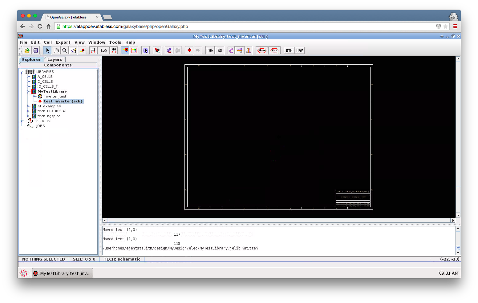
You will get an empty schematic sheet with a printable frame

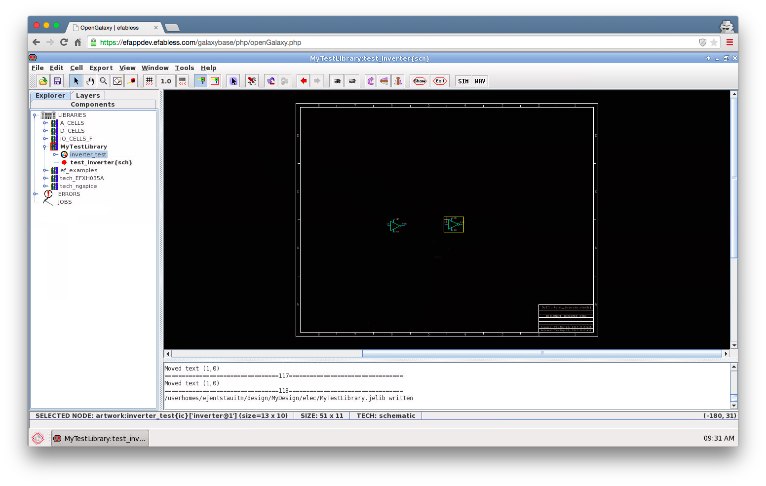
Now drag and drop the inverter we just created to construct a circuit to simulate.

Extra components are available from the ‘Components’ tab in the explorer bar, such as the ground symbol.

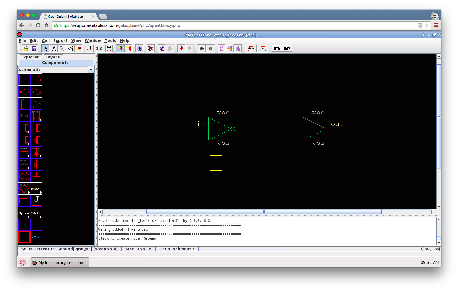
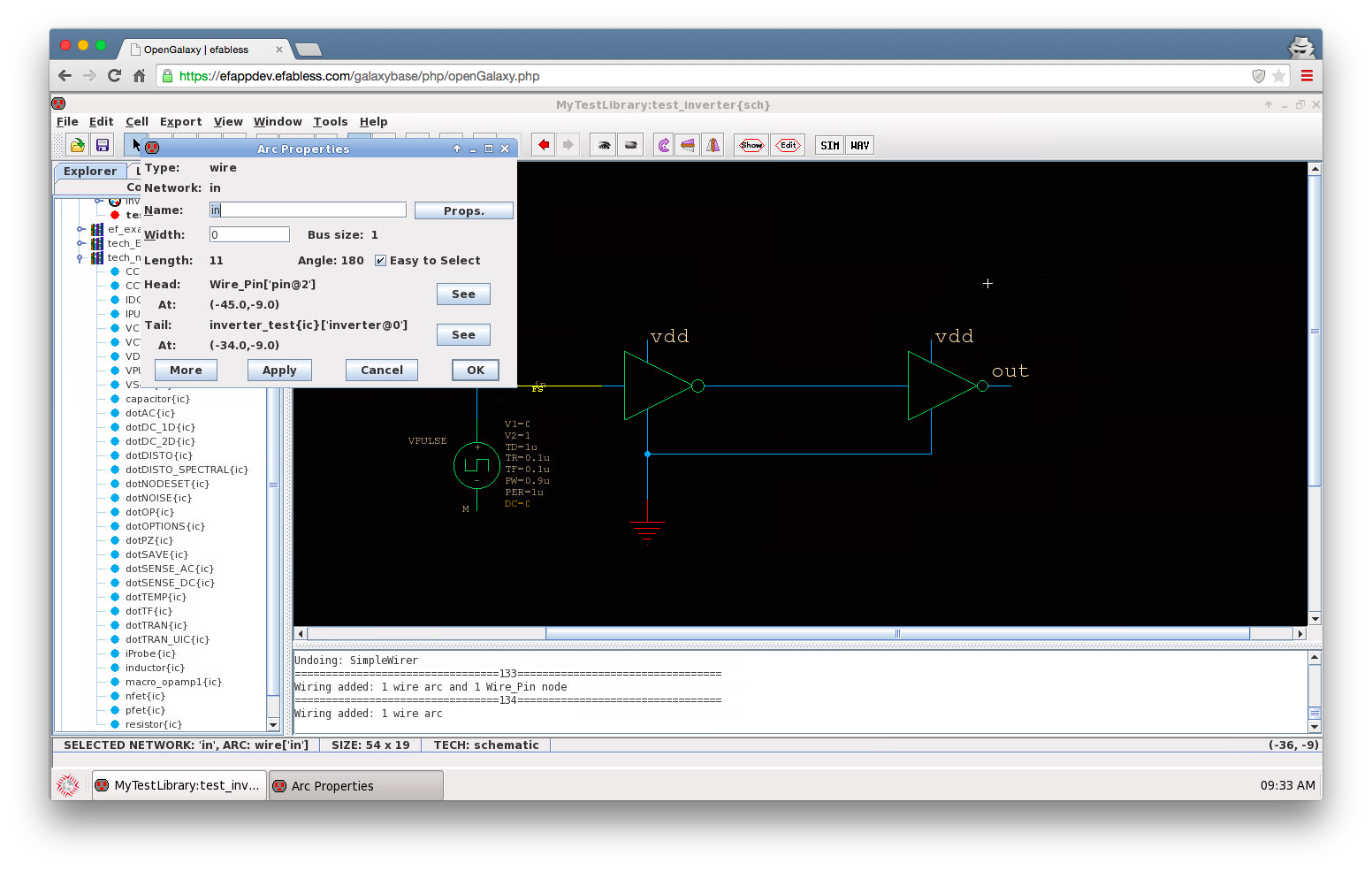
Wires can be named by double clicking on them, typing in a name (the name is preserved with netlisting to a spice compatible netlist)

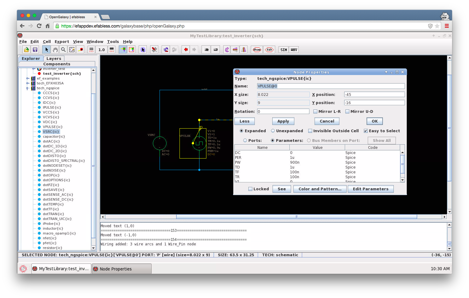
After the test schematic is complete (added the required voltage sources for transient simulation), adjust the voltage sources by double clicking on each

In the parameters section (make sure the parameters radiobox is selected), adjust the source parameters as needed, in this case we are using a pulse source that toggled between 0V and 3.3V, with rise/fall times of 100ps, an initial delay of 100ps. The power supply is set to 3.3V.

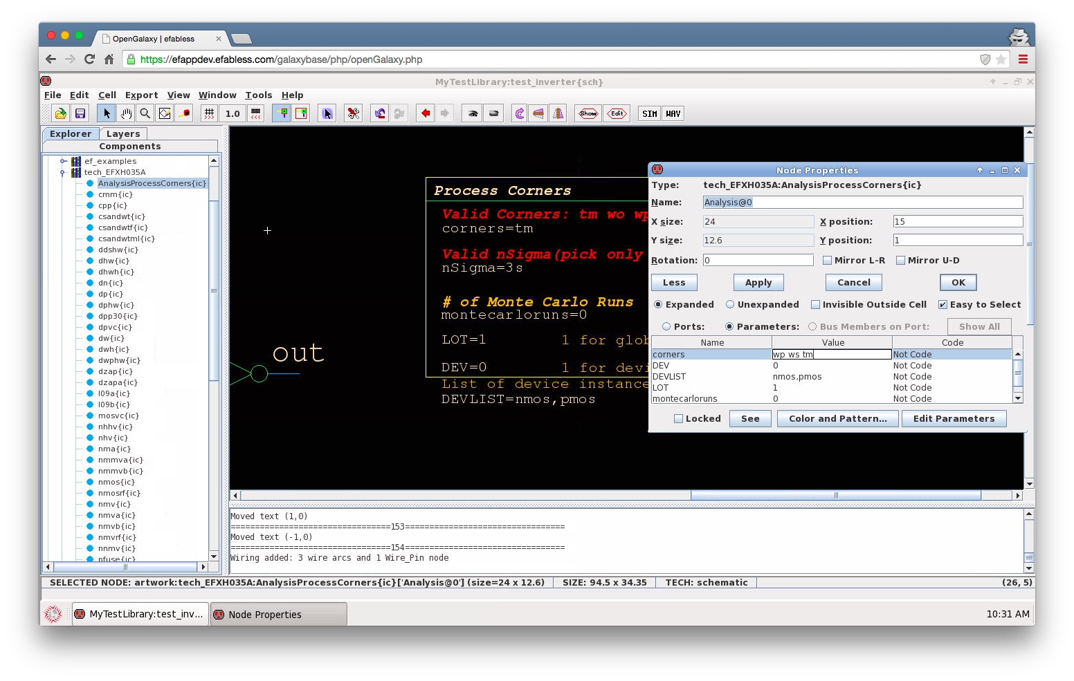
To prepare the sheet for simulation we need to identify process technology parameters, from the tech_EFXH035A library on the left drag the ‘AnalysisProcessCorners’ icon into the sheet. This instance identifies the process corners and models required to simulate the inverter.

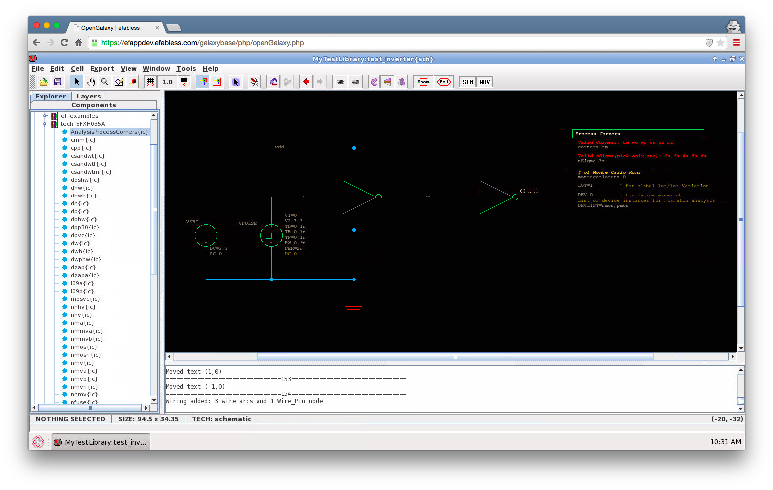
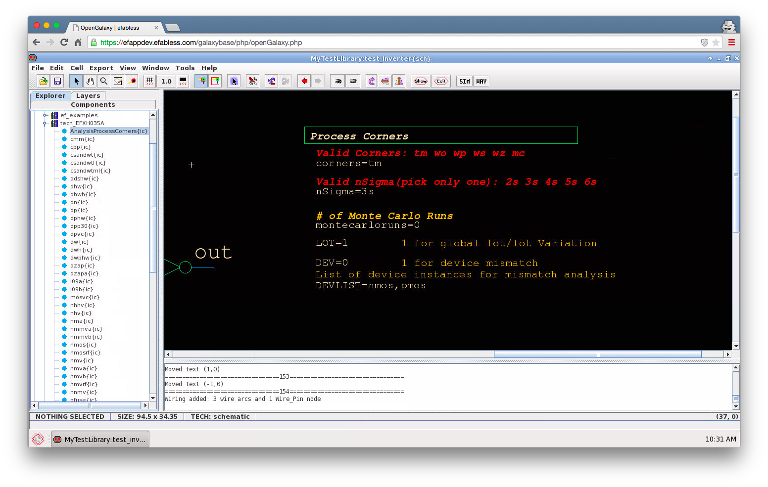
To choose which process parameters to simulate double click the AnalysisProcessCorners symbol, in this case we are going to simulate multiple process corners

wp: worst case power

ws: worst case speed

tm: typical corner

the models are set to 3 sigma simulations by default, this can be adjusted as well

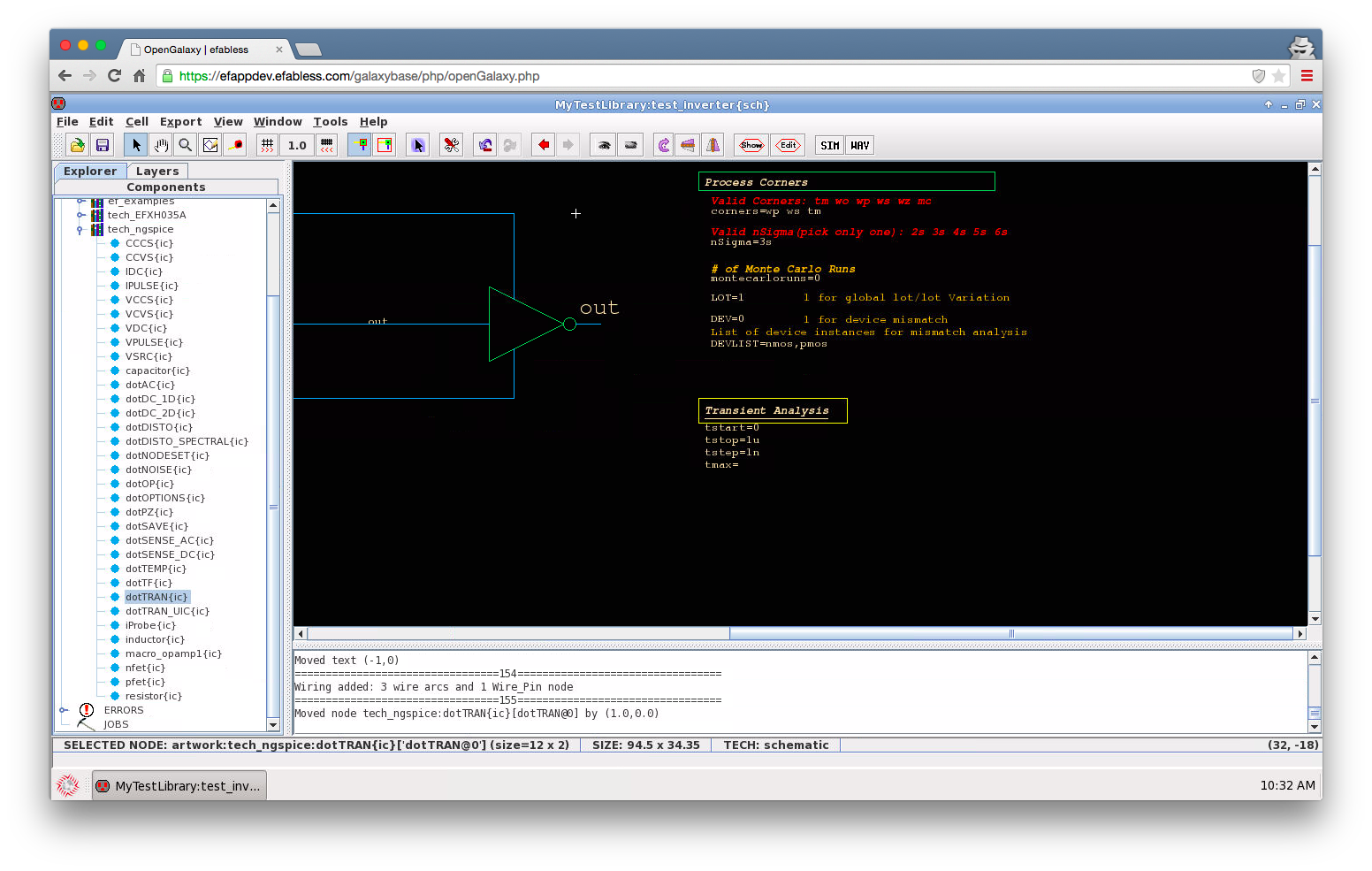
Now we need to add the simulate control statement, the tech_ngspice library contains multiple symbols that are prefixed with ‘dot’, these can be used for simulation control and other options. In this case we are going to make a transient simulation, we use the dotTRAN icon.

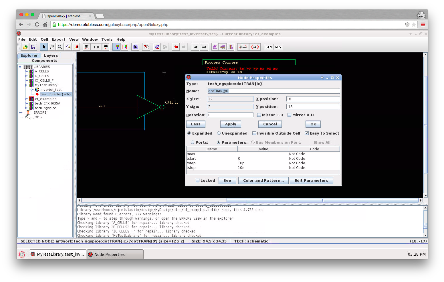
To adjust the transient simulation parameters double click on the Transient Analysis box, and fill in the simulation parameters. In this case we are simulating for 10ns with a default step of 10ps

OPTIONAL: We can add extra spice control code to any sheet, got to the Components tab in the explorer bar, select ‘Misc’ and choose ‘Spice Code’ from the pop-up menu

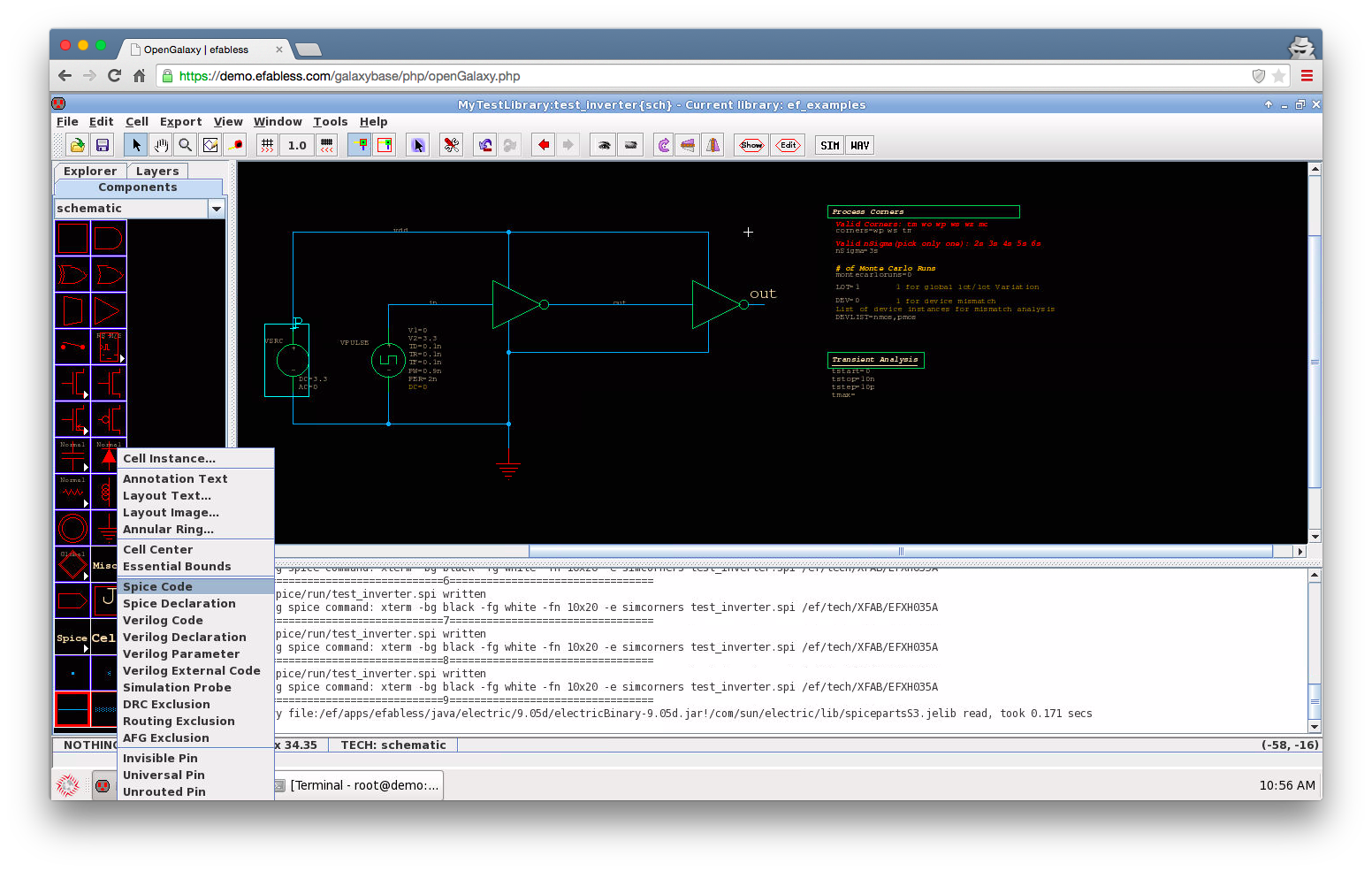
You can place the spice code anywhere in the schematic, in this case we are adding “.option filetype=ascii” to set ngspice to output ASCII raw files

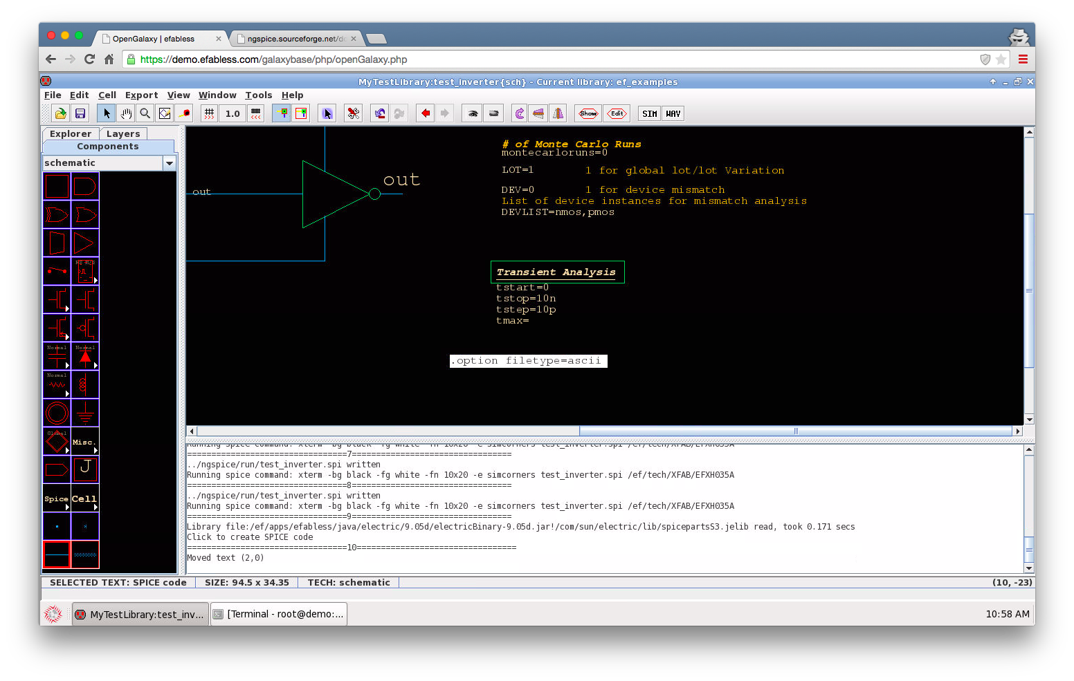
Now the schematic is complete, click the ‘SIM’ button, it’s near the right-side in the toolbar. Simulation will start automatically.

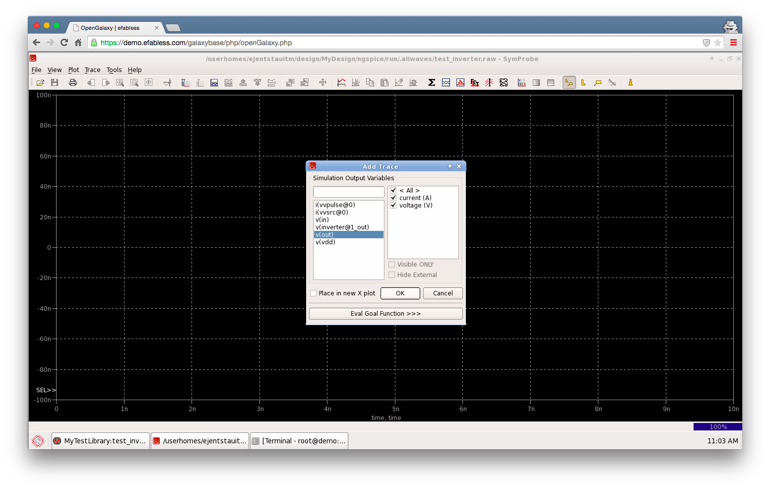
After simulation is complete start the waveform viewer (toolbar button to the right of SIM) (symprobe in this case) will be loaded with the first simulated corner on the list. You can view waveforms by clicking on the ‘Trace’ button highlighted.

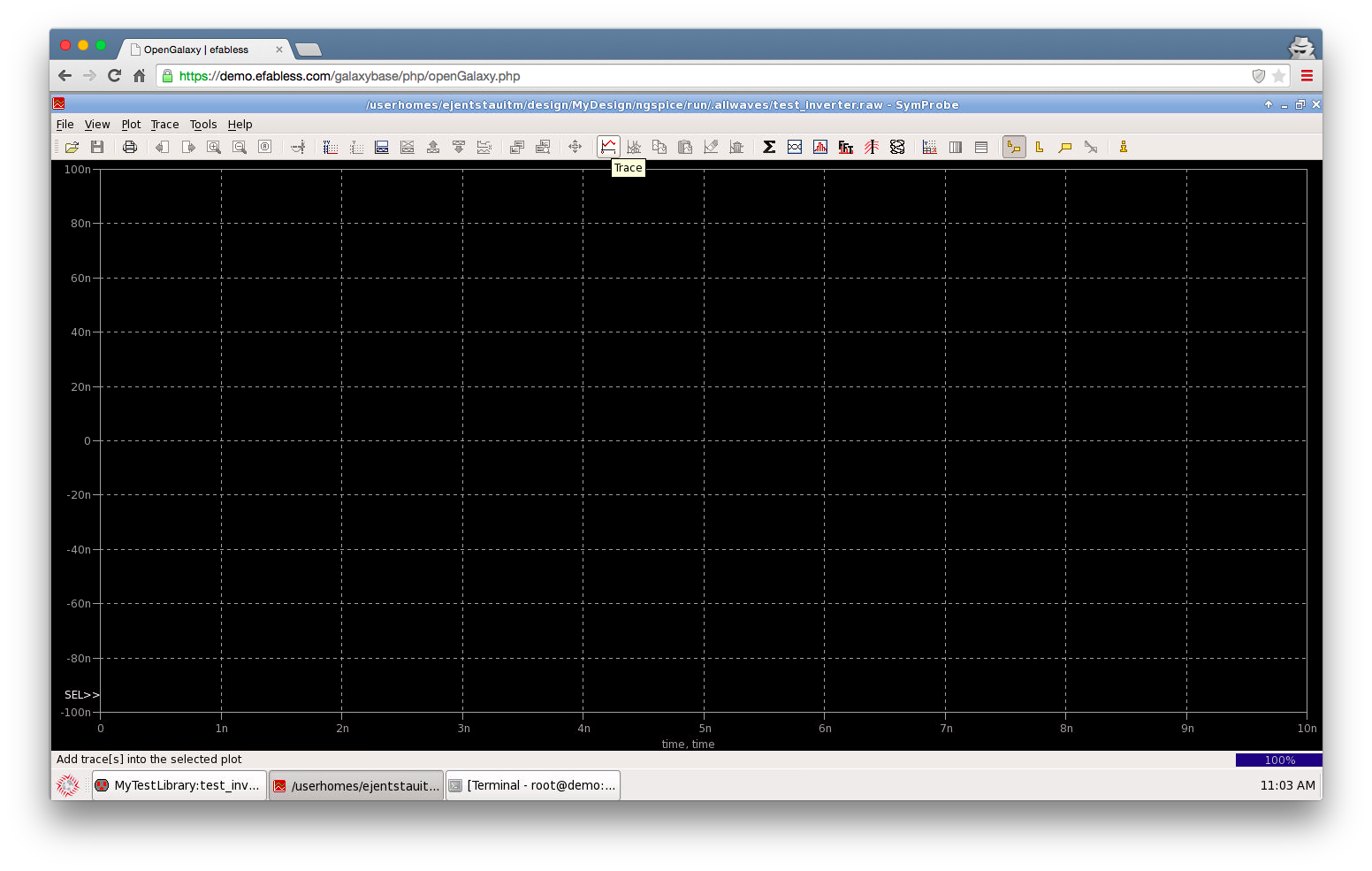
You can add waveforms to overlay, in this case we are selecting the input and output voltages of the inverter